Louvain and leiden algorithm

Clustering algorithm

For the default usage of clustering algorithm in scanpy, there are 4 settings.

1. Original Louvain
2. Louvain with multilevel refinement
3. SLM
4. Leiden algorithm

Louvain and leiden

From Louvain to Leiden: guaranteeing well-connected communities - Scientific Reports

Community detection - Tim Stuart

Clustering with the Leiden Algorithm in R (r-project.org)

Community detection is often used to understand the structure of large and complex networks.

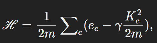
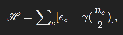
Constant Potts Model (CPM) which over comes some limitations of modularity:

The new algorithm integrates several earlier improvements, incorporating a combination of smart local move15, fast local move16,17and random neighbour move18.

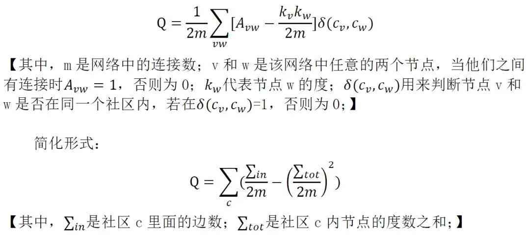
Modularity python code practice

import numpy as np

data = np.matrix([[1,0,0],[0,1,1],[1,0,1]])
label = np.matrix([[0,1],[1,0],[0,1]])
# calculate the connectivity of the matrix
m = np.sum(np.sum(data, axis=0)) /2
print(f"The network has totally %d connections" % m)
## The network has totally 2 connections ##
# calculate the degree of each node
k = np.sum(data, axis=1)
print(f"The degree of each node is {k}")
## The degree of each node is [[1]
##  [2]
##  [2]]
# calculate the modularity matrix
b = data - np.multiply(np.tile(k, (1,3)), np.tile(k.T, (3,1))) / (2*m)
print(f"The modularity matrix is {b}")
## The modularity matrix is [[ 0.8 -0.4 -0.4]
## [-0.4  0.2  0.2]
## [ 0.6 -0.8  0.2]]
# calculate the modularity
q = 1/(2*m) * np.trace(label.T*b*label)
print(f"The modularity is {q}")
## The modularity is 0.27999999999999997

The value of modularity is in [-1, 1], and if all of the nodes are allocated into 1 community the modularity is 1, while if each of the node is individually community the modularity is -1. When the value is in 0.3 ~ 0.7, the performance is good.

Louvain Algorithm process

Two stages:

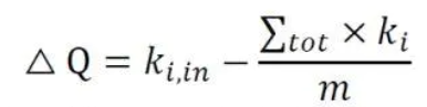
1. To allocate each node as one independent community, and then calculate the current modularity. For node i, try to delete node i form its own community rather than has the same community with node j and calculate the outcome modularity. Now, we got the increasment of the modularity comparing the two steps. For loop each node j in whole community, move the node i to the community with the highest increasment of modularity. The figure shows the equation of the increasment of modularity.

1. Aggregating the network in the first step, try to reconsturct the whole network.

In this stage we essentially collapse communities down into a single representative node, creating a new simplified graph. To do this we just sum all the edge weights between nodes of the corresponding communities to get a single weighted edge between them, and collapse each community down to a single new node. Once aggregation is complete we restart the local moving phase, and continue to iterate until everything converges down to one node. This aspect of the Louvain algorithm can be used to give information about the hierarchical relationships between communities by tracking at which stage the nodes in the communities were aggregated.

Limitations and Improvements on Louvain

Modularity suffers from a difficult problem known as the resolution limit, where there is a minimal community size that not able to be resovled by optimizing modularity. The community with size smaller than the minimal size could not be identified through optimizing modularity.

Constant Potts Model (CPM) which is an alternative objective function for community detection algorithm. The object of CPM is to maximize the internal connection edges in a community, while keep the community size small, and the constant parameter balances the two characteristics. The CPM could better split into two communities when the link density between the community is lower than constant, and the constant here acts like resolution. Higher constant will result in fewer communities.

Smart Local Move (SLM) find that the original louvain has difficults to split the communities once they are merged even though the total modularity would gain more. SLM tries to add a step which is to consider each sub-network as a new community and re-apply local movement to them after running local movement. And any sub-networks found in this step could treat as a different communities in aggregation step.

Random Moving means that choosing a random neighbor node in each moving stage rather than iteratively for all node. The reason is that in most of the time, the community with neighbors could gain more modularity. And the random move also help the algorithm more explorative and it could detect better community structures.

Louvain pruning keeps track of a list of nodes that have the potential to change the community which would reduce much more time in stage I.

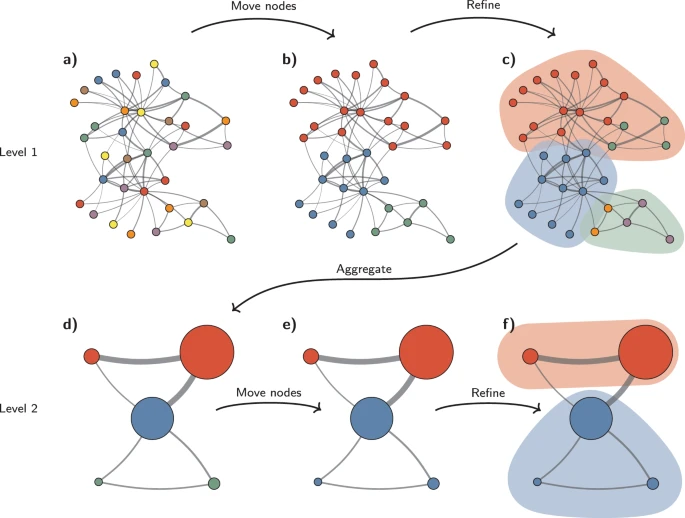
Leiden Algorithm process

The Leiden algorithm consists of three phases: (1) local moving of nodes, (2) refinement of the partition and (3) aggregation of the network based on the refined partition, using the non-refined partition to create an initial partition for the aggregate network.

The refinement step allows badly connected communities to be split before creating the aggregate network. This is very similar to what the smart local moving algorithm does. As far as I can tell, Leiden seems to essentially be smart local moving with the additional improvements of random moving and Louvain pruning added.