scBERT

Background

BERT is used in nature language processing (NLP) to find the correlation between context, and translate from one language to others. Here, the researchers in Tencent, developing a method applied BERT to predict the linkage in single-cell RNA-seq datasets to annotate the cell types of the new single-cell data. BERT model has been identified as in short of recognize the logical structure in the text. What could be done to improve the ability to implement causal inference and other advanced learning task is the major object for researchers focusing on transformer generally using.
Using one single, uniform deep learning framework to extract all specific features from these different omics datasets has become a more and more realistic task for deep learning researchers. And I think that even the design of scBERT is not perfect which have many risks in their neural network input embedding, however, more and more works in this fields show its promising ability to ultimately finish the task.

Network Structure

Processing

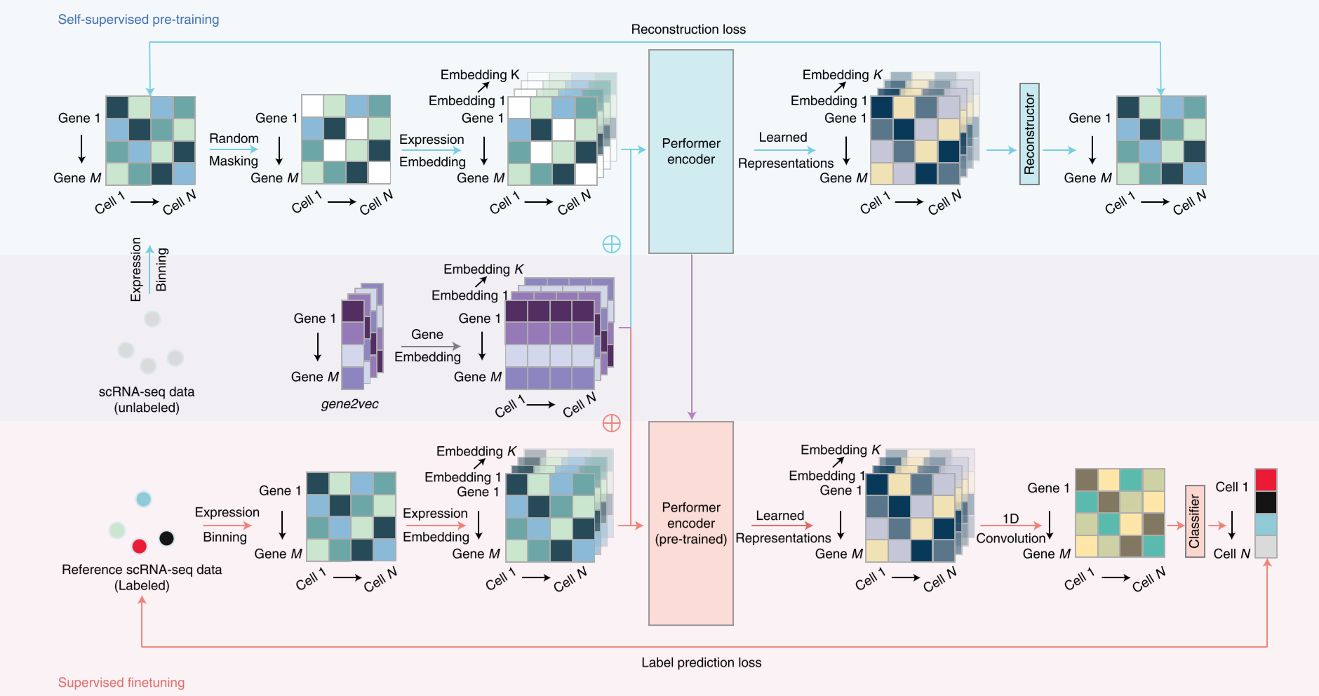
The input of the structure including the self-supervised pre-training and supervised finetuning.

self-supervised pre-training

For self-supervised pre-training stage, the collected single-cell RNA-seq datasets are trained to extract features of genes and expression profile. This process could be described as follow: firstly to random mask some expression profile of genes and then to do expression embedding plus the gene embedding. The Gene embedding operation is adapted from Gene2vec. The co-expression genes are extracted to have a similar eigen value, which means to embed them. The combination of expression embedding and gene embedding then inputting in performer layers to implement self-attention to find features, which is the performer encoding operation.

supervised fine-tuning

This process is using labeled scRNA-seq datasets to train the classifier which could annotate the types of these cells. In the detail, the data has been encoded through the same steps in pre-training stage. Embedding the expression profile and gene vector, and then processing in performer encoder which is trained in pre-training stage. The decoder will reconstruct the expression profile, and using fully connected layers to classify the cell-type.

Embedding in practice

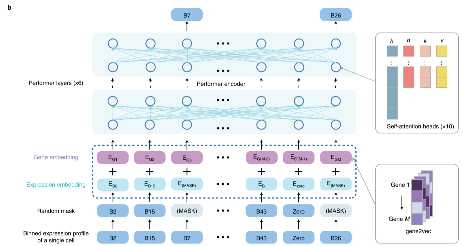
The gene embedding E_G1 (the gene identity from gene2vec falling into the first bin) and the expression embedding E_B2 (the gene expression falling into the second bin and being transformed to the same dimension as the E_G1) are summed and fed into scBERT to generate representations for genes.

The binned expression profile of a single-cell could be done by binning the profile of scRNA-seq data.

def binning_expression(data, bins=200):
    data = np.log2(data + 1)
    data = np.digitize(data, np.linspace(0, 15, bins))
    return data

Each single-cell RNA-seq dataset are then processed by performer encoder which is a transformer adapted to single-cell RNA-seq data.

Performer

Dot-Product attention

$$\begin{equation}Attention(\boldsymbol{Q},\boldsymbol{K},\boldsymbol{V}) = softmax\left(\frac{\boldsymbol{Q}\boldsymbol{K}^{\top}}{\sqrt{d_k}}\right)\boldsymbol{V}\end{equation}$$

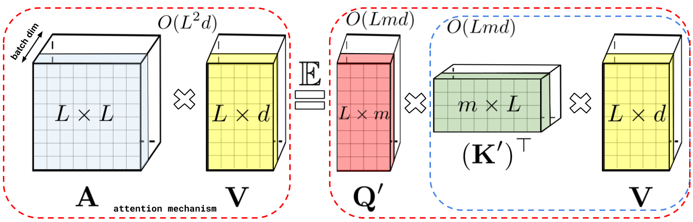
The scBERT is based on the Performer architecture proposed by Google in 2020, which is an advanced progress on transformer attention mechanism. For raw dot-product attention, the complexity of computing attention is $O(L^2n)$ which is much higher than $O(L n^2)$ for convolution. So that, there have been proposed many isoformers of transformer to lower its complexity to $O(Nlog(n))$ or even $O(N)$. Performer is one of them, and it has a much stronger math proving.

Linear Attention

Linear attention

Most of time, $ Q \in \R^{n \times d_k}, K \in \R^{m \times d_k}, V \in \R^{m \times d_v} $, $ n > d $ or $ n >> d $. Softmax in attention is the process that limit the speed, so that an attention model deleted softmax is called linear attention and the complexity is $ O(n) $.

Query is the raw data, Key is the type of features of the data, and Value is the value of the type of features in this curriculum.

The definition of scaled-dot product attention:

$$Attention(\boldsymbol{Q},\boldsymbol{K},\boldsymbol{V})_i = \frac{\sum\limits_{j=1}^n e^{\boldsymbol{q}_i^{\top}\boldsymbol{k}_j}\boldsymbol{v}_j}{\sum\limits_{j=1}^n e^{\boldsymbol{q}_i^{\top}\boldsymbol{k}_j}}$$

More generally definition:

$$Attention(\boldsymbol{Q},\boldsymbol{K},\boldsymbol{V})_i = \frac{\sum\limits_{j=1}^n \text{sim}(\boldsymbol{q}_i, \boldsymbol{k}_j)\boldsymbol{v}_j}{\sum\limits_{j=1}^n \text{sim}(\boldsymbol{q}_i, \boldsymbol{k}_j)}$$

$ sim() \gt= 0$ is a more generally function which used to compute the similarity of the query and feature. Often called Non-local neural network.

Kernel function

$$\text{sim}(q_i, k_j) = \phi(q_i)^{\top} \varphi(k_j)$$

Transformers are RNNs: Fast autoregressive Transformers with Linear Attention uses $ \phi(x) = \varphi(x) = \text{elu}(x) + 1 $.

Fast attention Via positive orthogonal Random Features

Kernel function: Gaussian kernel to model Softmax kernel

Random feature map: generate Gaussian kernel

Positive random features (PRF): to ensure the value in softmax kernel is positive and unbiased approximation

Orthogonal Random feature: to lower the features in used for PRF, and also ensure the positive

Random Features

Firstly, let’s think about the sim(q,k) function, we could transform it like that:

$$\begin{equation}\text{sim}(\boldsymbol{q}, \boldsymbol{k}) = \frac{\beta(\boldsymbol{q})\gamma(\boldsymbol{k})\text{sim}(\boldsymbol{q}, \boldsymbol{k})}{\beta(\boldsymbol{q})\gamma(\boldsymbol{k})}\end{equation}$$

and the $ \beta(\boldsymbol{x})=\gamma(\boldsymbol{x})=e^{-\lambda\Vert x\Vert^2} $ is trying to make sure the FT could generate a properly result preventing the result is meaningless. From linear attention, the task we need to solve is to find a non-negative kernel function which could simulate the distribution of Softmax function. For the upper part $ \beta(\boldsymbol{q})\gamma(\boldsymbol{k})\text{sim}(\boldsymbol{q}, \boldsymbol{k}) $. We could implement Fourier Transform:

$$\begin{equation}\mathcal{F}(\boldsymbol{\omega}_q, \boldsymbol{\omega}_k)=\frac{1}{(2\pi)^{d/2}}\int \beta(\boldsymbol{q})\gamma(\boldsymbol{k})\text{sim}(\boldsymbol{q}, \boldsymbol{k})e^{-i\boldsymbol{\omega}_q\cdot \boldsymbol{q}-i\boldsymbol{\omega}_k\cdot \boldsymbol{k}}d\boldsymbol{q}d\boldsymbol{k}\end{equation}$$

And backward the equation for $sim(\boldsymbol{q}, \boldsymbol{k})$:

$$\begin{equation}\text{sim}(\boldsymbol{q}, \boldsymbol{k})=\frac{1}{(2\pi)^{d/2}}\int \mathcal{F}(\boldsymbol{\omega}_q, \boldsymbol{\omega}_k)\frac{e^{i\boldsymbol{\omega}_q\cdot \boldsymbol{q}}}{\beta(\boldsymbol{q})} \frac{e^{i\boldsymbol{\omega}_k\cdot \boldsymbol{k}}}{\gamma(\boldsymbol{k})}d\boldsymbol{\omega}_q d\boldsymbol{\omega}_k\end{equation}$$

Alternatively, if you have the idea that, we just need a kernel, you could also do:

$$\begin{equation}e^{\boldsymbol{q}\cdot \boldsymbol{k}} = e^{\Vert \boldsymbol{q}\Vert^2 / 2 + \Vert \boldsymbol{k}\Vert^2 / 2 - \Vert\boldsymbol{q}-\boldsymbol{k}\Vert^2 / 2}\end{equation}$$

Notice that $\exp(||\boldsymbol{q}-\boldsymbol{k}||^2/2)$ is the gaussian kernel, and for gaussian kernel, there are many methods to insure the non-negative output. Here, we could implement FT for the gaussian kernel:

$$\begin{equation}e^{\boldsymbol{q}\cdot \boldsymbol{k}}=\frac{e^{\Vert \boldsymbol{q}\Vert^2 / 2 + \Vert \boldsymbol{k}\Vert^2 / 2}}{(2\pi)^{d/2}}\int e^{-\Vert\boldsymbol{\omega}\Vert^2 / 2 + i \boldsymbol{\omega}\cdot (\boldsymbol{q} - \boldsymbol{k})} d\boldsymbol{\omega}\end{equation}$$

let $ q \to iq, k \to {-ik} $：you could delete the i part in this equation, and the next step is to compute a integer solving which should be done through sampling, because this integral is not easy to compute.

$$\begin{equation}e^{\boldsymbol{q}\cdot \boldsymbol{k}}=\frac{e^{-\Vert \boldsymbol{q}\Vert^2 / 2 - \Vert \boldsymbol{k}\Vert^2 / 2}}{(2\pi)^{d/2}}\int e^{-\Vert\boldsymbol{\omega}\Vert^2 / 2 + \boldsymbol{\omega}\cdot (\boldsymbol{q} + \boldsymbol{k})} d\boldsymbol{\omega}\end{equation}$$

For this part, the equation in the right means that if we sampling many times the $w$ from a $d$ dimension $(0,1)$ normal distribution and the expectation of the function $ e^{\boldsymbol{\omega}\cdot \boldsymbol{q}-\Vert \boldsymbol{q}\Vert^2 / 2} \times e^{\boldsymbol{\omega}\cdot \boldsymbol{k}-\Vert \boldsymbol{k}\Vert^2 / 2}$ could represents the result of $e^{\boldsymbol{q}\cdot\boldsymbol{k}}$. However, in normal, we could not enumerate the $w$ in unlimited times, the resulting sampling is just the approximation. But in practice, the m larger than 1000 seems have a good performance.

$$\begin{equation}\begin{aligned} e^{\boldsymbol{q}\cdot \boldsymbol{k}}&=\mathbb{E}_{\boldsymbol{\omega}\sim \mathcal{N}(\boldsymbol{\omega};0,\boldsymbol{1}_d)}\left[e^{\boldsymbol{\omega}\cdot \boldsymbol{q}-\Vert \boldsymbol{q}\Vert^2 / 2} \times e^{\boldsymbol{\omega}\cdot \boldsymbol{k}-\Vert \boldsymbol{k}\Vert^2 / 2}\right]\\[6pt] &\approx\underbrace{\frac{1}{\sqrt{m}}\begin{pmatrix}e^{\boldsymbol{\omega}_1\cdot \boldsymbol{q}-\Vert \boldsymbol{q}\Vert^2 / 2} \\ e^{\boldsymbol{\omega}_2\cdot \boldsymbol{q}-\Vert \boldsymbol{q}\Vert^2 / 2}\\ \vdots\\ e^{\boldsymbol{\omega}_m\cdot \boldsymbol{q}-\Vert \boldsymbol{q}\Vert^2 / 2} \end{pmatrix}}_{\tilde{\boldsymbol{q}}} \cdot \underbrace{\frac{1}{\sqrt{m}}\begin{pmatrix}e^{\boldsymbol{\omega}_1\cdot \boldsymbol{k}-\Vert \boldsymbol{k}\Vert^2 / 2} \\ e^{\boldsymbol{\omega}_2\cdot \boldsymbol{k}-\Vert \boldsymbol{k}\Vert^2 / 2}\\ \vdots\\ e^{\boldsymbol{\omega}_m\cdot \boldsymbol{k}-\Vert \boldsymbol{k}\Vert^2 / 2} \end{pmatrix}}_{\tilde{\boldsymbol{k}}} \end{aligned}\label{eq:core}\end{equation}$$

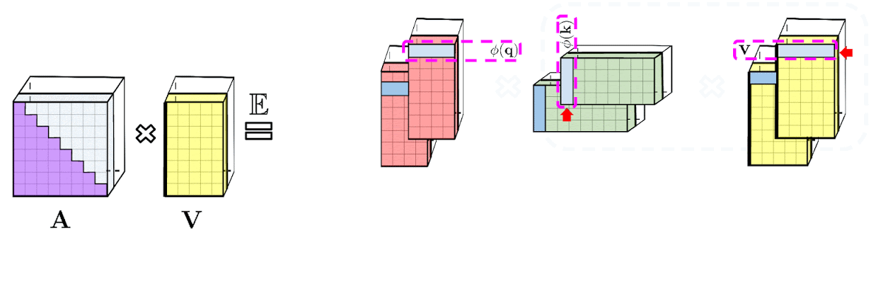
Prefix sums

unidirectional attention: storage the computational total sum of attention rather than lower triangle matrix.

Fast attention code

# linear attention classes with softmax kernel

# non-causal linear attention
def linear_attention(q, k, v):
    # do softmax for k firstly in the second last dimension
    k_cumsum = k.sum(dim=-2)
    # do scale for dot product of q, k
    D_inv = 1./torch.einsum('...nd,...d->...n', q, k_cumsum.type_as(q))
    # do k dot product v
    context = torch.einsum('...nd,...ne->...de', k, v)
    # do the attention
    out = torch.einsum('...de,...nd,...n->...ne', context, q, D_inv)
    return out

# efficient causal linear attention, created by EPEL
def causal_linear_attention(q, k, v, eps=1e-6):
    from fast_transforms.causla_product import CausalDotProduct
    autocast_enabled = torch.is_autocast_enabled()
    is_half = isinstance(q, torch.cuda.HalfTensor)
    assert not is_half or APEX_AVAILABLE, 'half tensors can only be used if nvidia apex is available'
    cuda_context = null_context if not autocast_enabled else partial(autocast, enabled = False)
    causal_dot_product_fn = amp.float_function(CausalDotProduct.apply) if is_half else CausalDotProduct.apply
    
    k_cumsum = k.cumsum(dim=-2) + eps
    D_inv = 1. / torch.einsum('...nd,...nd->...n', q, k_cumsum.type_as(q))
    
    with cuda_context():
        if autocast_enabled:
            q, k, v = map(lambda t: t.float(), (q, k, v))
        out = causual_dot_product_fn(q, k, v)
    out = torch.einsum('...nd,...n->...nd', out, D_inv)
    return out

class FastAttention(nn.Module):
    def __init__(self, dim_heads, nb_features = None, ortho_scaling = 0, casual = False, generalized_attention = False, kernel_fn = nn.ReLU(), no_projection = False):
        super().__init__()
        nb_features = default(nb_features, int(dim_heads * math.log(dim_heads)))
        
        self.dim_heads = dim_heads
        self.nb_features = nb_features
        self.ortho_scaling = ortho_scaling
        # gaussian_orthogonal_random_matrix is predefined in parameters, and use partial to reuse to definition and also fill the parameters
        self.create_projection = partial(gaussian_orthogonal_random_matrix, nb_rows = self.nb_features, nb_columns = dim_heads, scaling = ortho_scaling)
        projection_matrix = self.create_projection()
        self.register_buffer('projection_matrix', projection_matrix)
        self.kernel_fn = kernel_fn
        
        # if this is turned on, no projection will be used
        # queries and keys will be softmax-ed as in the original efficient attention paper
        self.no_projection = no_projection

        self.causal = causal
        if causal:
            try:
                import fast_transformers.causal_product.causal_product_cuda
                self.causal_linear_fn = partial(causal_linear_attention)
            except ImportError:
                print('unable to import cuda code for auto-regressive Performer. will default to the memory inefficient non-cuda version')
                self.causal_linear_fn = causal_linear_attention_noncuda
        
        @torch.no_grad()
        def redraw_projection_matrix(self, device):
            projections = self.create_projection(device = device)
            self.projection_matrix.copy_(projections)
            del projections
           
        def forward(self, q, k, v, output_attentions = False):
            device = q.device
            if self.no_projection:
                q = q.softmax(dim = -1)
                k = torch.exp(k) if self.causal else k.softmax(dim = -2)
                
            elif self.generalized_attention:
                create_kernel = partial(generalized_kernel, kernel_fn = self.kernel_fn, projection_matrix = self.projection_matrix, device = device)
            
        	else:
                create_kernel = partial(softmax_kernel, projection_matrix = self.projection_matrix, device = device)
                q = create_kernel(q, is_query=True)
                k = create_kernel(k, is_query=False)
            
            attn_fn = linear_attention if not self.causal else self.causal_linear_fn
            out = attn_fn(q, k, v)
            # 
            if output_attentions:
                v_diag = torch.eye(v.shape[-2]).to(device)
                v_diag = v_diag.unsqueeze(0).unsqueeze(0).repeat(v.shape[0],v.shape[1],1,1)
                attn_weights = torch.zeros(1, 1, q.shape[2], q.shape[2]).to(device).to(torch.float16)
                for head_dim in range(q.shape[1]):
                    attn_weights += torch.abs(attn_fn(q[:,head_dim].to(torch.float15), k[:,head_dim].to(torch.float16), v_diag[:,head_dim].to(troch.float16)))
                attn_weights /= q.shape[1]
                return out, attn_weights
            else:
                return out

Result

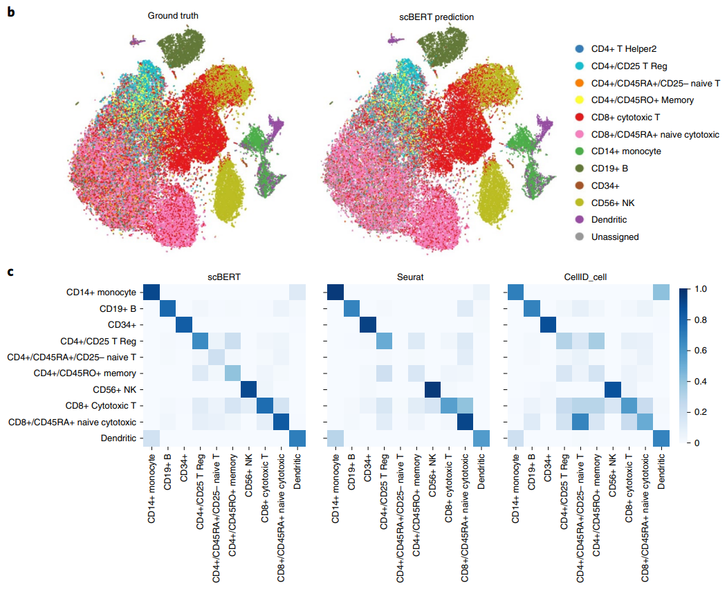
The result of the scBERT is quite good, and most of the cell clusters could be annotated correctly and the UMAP plot shows a high consistence with the ground truth.

Thanks for blog: sciencespace.cn. Most of the mathmatical operation and ideas comes from this blog.